1、CRDB的执行计划大致与PG相当， 语法增加了distsql关键字，用于查询分布式的执行计划

2、提供了网页链接进行图形化展示，更加清晰明了

CR的执行计划

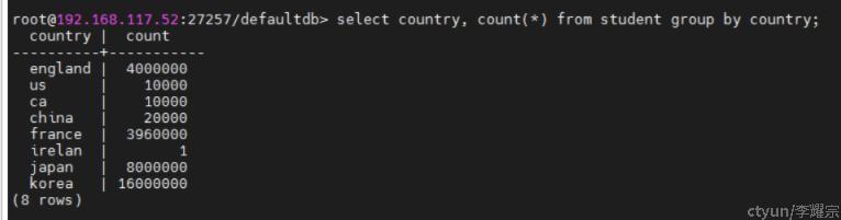
上述的读场景和写场景是针对一个表只有一个range的场合进行的简单描述，正如我们在章节一中的student表，3200w行数据，分成了7个range。

那么如果我们查询其中的某些数据，需要访问哪些range？

这里可以依赖CR的查看执行计划功能来了解查询的具体过程。所有关系型数据库都具备执行计划这个概念，简单地说，就是展示数据库引擎是通过何种途径去查询数据。

比如现在已知student表中的数据分布如下：

现在我通过如下命令查看“查询irelan的数据的执行计划”

explain analyze (distsql) select * from student where country = 'irelan';

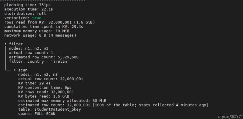
由上图可知

planning time：生成执行计划的耗时为751us

execution time：执行上述查询的耗时为22.1s

row read from KV：从KV中读取的行数32000001（1.6GB）

cumulative time spent in KV： 累计在KV的读取耗时29.4s （多节点耗时累加，因为是并行所以实际耗时小于该值）

maximum memory usage： 最大内存消耗 10MB

filter：过滤器

nodes：涉及的节点（如上图，所有节点都访问到了）

actual row count ： 1

estimated row count : 5329600 预估的行数

filter： 过滤条件

sacn：子操作，扫描，执行了FULL SCAN，全表扫描，总计扫描32000001行，KV耗时29.4秒，KV读取数据量1.6GB，通过student@student_pkey进行全表扫描。

CR还提供了一个网页，观察图形化的执行计划

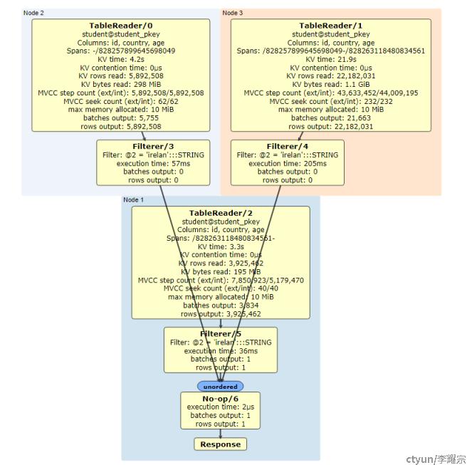
如图所示，Node1、Node2和Node3分别执行全表扫描，并将得到的数据流经过Filterer @2 = 'irelan':::STRING 过滤，得到的结果发送到Node1进行No-op6 汇总，得到输出行数为1，并最终反馈Response给客户端。

整个过程中，耗时最多的是Node3进行KV读取，耗时21.9秒；Node3的Filter耗时205ms，其他环节耗时基本上是10+毫秒级别，汇总耗时为2us，总耗时为22.1秒。

PS：关于任意一个节点是如何知道数据range的分布情况，可以参考官网架构文档中的Distributed Layer章节中关于Meta range的说明。

CR的索引

上面的查询虽然带了查询条件 where country = 'irelan';， 但是由于没有合适的索引，因此进行了全表扫描。像普通关系型数据库一样，可以通过索引来提高查询效率。同时，由于CR的索引也是通过KV存储的，因此如果使用恰当的索引方式，甚至可以进一步提高查询效率。

比方说，执行如下SQL进行索引创建：

CREATE INDEX ON student (country) STORING (id);

该命令的意思是针对student表，基于country字段进行索引，并且在索引中存储id字段的数据。

下面我们看看以下两个查询的执行计划

explain analyze (distsql) select id,country from student where country = 'irelan';

-----------------------------------------------------------------------------------------------------
  planning time: 809µs
  execution time: 31ms
  distribution: local
  vectorized: true
  rows read from KV: 1 (50 B)
  cumulative time spent in KV: 30ms
  maximum memory usage: 20 KiB
  network usage: 0 B (0 messages)

  • scan
    nodes: n1
    actual row count: 1
    KV time: 30ms
    KV contention time: 0µs
    KV rows read: 1
    KV bytes read: 50 B
    estimated max memory allocated: 20 KiB
    estimated row count: 0 (<0.01% of the table; stats collected 9 minutes ago)
    table: student@student_country_idx
    spans: [/'irelan' - /'irelan']

Time: 34ms total (execution 33ms / network 1ms)

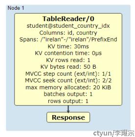
只经过节点1，即可返回数据，通过student@student_country_idx进行查询，访问了新建的索引student_country_idx的range即可得到结果。

explain analyze (distsql) select id,country,age from student where country = 'irelan';

-------------------------------------------------------
  planning time: 654µs
  execution time: 33ms
  distribution: local
  vectorized: true
  rows read from KV: 2 (81 B)
  cumulative time spent in KV: 32ms
  maximum memory usage: 50 KiB
  network usage: 0 B (0 messages)

  • index join
  │ nodes: n1
  │ actual row count: 1
  │ KV time: 30ms
  │ KV contention time: 0µs
  │ KV rows read: 1
  │ KV bytes read: 31 B
  │ estimated max memory allocated: 20 KiB
  │ estimated max sql temp disk usage: 0 B
  │ estimated row count: 0
  │ table: student@student_pkey
  │
  └── • scan
        nodes: n1
        actual row count: 1
        KV time: 2ms
        KV contention time: 0µs
        KV rows read: 1
        KV bytes read: 50 B
        estimated max memory allocated: 20 KiB
        estimated row count: 0 (<0.01% of the table; stats collected 48 seconds ago)
        table: student@student_country_idx
        spans: [/'irelan' - /'irelan']

Time: 35ms total (execution 35ms / network 1ms)

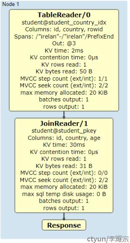
类似的查询，得到了不一样的执行计划，原因在于：经过索引查询得到id,country列的数据，但是无法得到age列，因此需要在索引中查到的rowid进一步利用主键student_pkey查询相应的表数据range，得到age字段的数据，总共访问了2个range合计2条KV。

因此，当节点数和range数线性扩展时，存在两种情况：

1、查询的字段在索引中完全包含，那么查询可以快速通过索引就得到结果，无须访问过多的range。由于索引组织的数据是有序的，因此也不用担心同一个user_id所涉及的数据会分散在所有range中。

2、查询的字段在索引中未能完全包含，仅能通过索引快速找到需要访问的数据range，并进一步查询。由于range被平均分布在所有节点中，理论上整个查询的耗时约等于最多range的节点的查询的耗时。数据分散在多个节点不一定比传统数据库（通过分片键分布数据）的效率低。（比方说，100w数据都由节点1去查询的耗时 VS 每个节点查询33w数据再汇总的耗时）